How it works · Core ideas
Optimization Problems in Calculus: How to Solve Them
How to solve optimization problems with derivatives: the steps, 4 worked examples with answers (fence, box, revenue, can), checks and common mistakes.
Checked against 4 sources (3 textbook, course or government) · By Ambient Math editors
The short answer. To solve an optimization problem, write the quantity you want to maximize or minimize as a function of one variable, using the constraint to eliminate the others, then find where its derivative is zero and check that point against the endpoints12. The best value occurs at a critical point or an endpoint2.
- Goal
- The largest or smallest value of a function subject to a constraint2
- Key move
- Use the constraint to turn 2 variables into 12
On this page
- What is an optimization problem?
- How to solve an optimization problem: the method
- Worked example 1: the fenced field
- How to be sure it is the maximum
- Worked example 2: the open-top box
- Worked example 3: revenue
- Worked example 4: the can
- Where students go wrong
- Practice problems in the style of section 4.7
- Beyond the classroom
- Where to go next
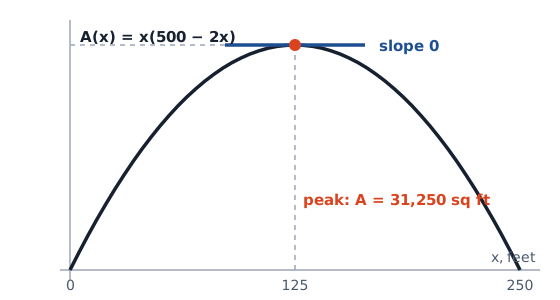
You have 500 feet of fence and a building to use as one side. Where do the posts go to enclose the most ground? Guess and you will be close. Differentiate and you will be exact. One common application of calculus is calculating the minimum or maximum value of a function1. Companies minimize production costs or maximize revenue, and in manufacturing it is often desirable to minimize the material used to package a product with a certain volume1.
What is an optimization problem?
In an optimization problem we look for the largest value or the smallest value that a function can take2. The version in this chapter adds a twist: we look for the largest or smallest value of a function subject to some kind of constraint2. A particular quantity is the one we want to maximize or minimize, and there is also some auxiliary condition that must be satisfied1.
The constraint is a condition, usually an equation, that must absolutely, positively be true no matter what our solution is2. In almost every problem one quantity is clearly indicated as having a fixed value, and that is the constraint2. In the wider world the subject is large: mathematical optimization is the selection of a best element, with regard to some criteria, from some set of available alternatives3. Calculus handles the smooth, continuous case. In the general approach, an optimization problem maximizes or minimizes a real function by choosing input values from within an allowed set3.
Optimization is the art of letting a constraint do the choosing, so the derivative only has one thing left to decide.
How to solve an optimization problem: the method
The first step in all of these problems, per the Lamar University notes, is to read the problem very carefully2. Then the next step is to identify the quantity to be optimized and the constraint2. The remaining steps:
- Draw it. If applicable, draw a figure and label all variables1. Sketching the situation will often help to arrive at the equations2.
- Name the target. Determine which quantity is to be maximized or minimized, and for what range of values of the other variables1.
- Write the target as a formula. Write a formula for the quantity to be maximized or minimized in terms of the variables1.
- Use the constraint to get one variable. There are 2 functions in every problem, the one to optimize and the constraint2. We know how to find the largest or smallest value of a function provided it has a single variable, so solve the constraint for one variable and substitute2.
- Find the domain. Both sides of a physical shape must be positive, for example1.
- Locate the optimum. This step typically involves looking for critical points and evaluating a function at endpoints1. The maximum value of a continuous function on a closed interval will occur at critical points and/or end points2.
- Answer the question asked. Do not forget to actually read the problem and give the answer that was asked for2.
Worked example 1: the fenced field
The problem is the standard one: enclose a rectangular field with a fence, with 500 feet of fencing material and a building on one side that needs no fence, and find the dimensions that enclose the largest area2. The source gives the answer, 250 by 1252. The arithmetic below is ours and gets there:
Worked example (our arithmetic): let x be the width of each of the 2 sides perpendicular to the building and y the side parallel to it1.
| Step | Arithmetic |
|---|---|
| Constraint (fence length) | 2x + y = 500, so y = 500 − 2x2 |
| Quantity to maximize (area) | A = x · y = x(500 − 2x) = 500x − 2x²2 |
| Domain | x > 0 and y > 0, so 0 < x < 2501 |
| Derivative | A′(x) = 500 − 4x1 |
| Critical point | 500 − 4x = 0, so x = 1251 |
| The other side | y = 500 − 2 × 125 = 2502 |
| Maximum area | 125 × 250 = 31,250 square feet2 |
| Endpoint check | A(0) = 0 and A(250) = 0, so the end points give zero area and cannot be the maximum2 |
| Second derivative | A″(x) = −4, negative everywhere, so the critical point is a maximum2 |
The diagram above is this function: the area climbs to its peak at x = 125 and falls back to 0, and the slope is zero exactly at the top2. The best field is half as wide as it is long.
How to be sure it is the maximum
Finding a critical point is not the same as proving it is the best one. The first derivative test identifies points that might be extrema, but it does not by itself say whether a point is a minimum, a maximum or neither3. A problem on a closed interval gets its answer by comparing the values at the critical points and at the endpoints2. Fermat’s work gives the underlying idea: optima of unconstrained problems are found at stationary points, where the first derivative is zero3. Fermat and Lagrange found calculus-based formulae for identifying optima3.
There are other checks. Not every problem has a closed interval with finite endpoints, and many of the functions are not continuous once reduced to one variable2. The second derivative can help: it is possible to use it to exclude values, though by itself that does not identify the optimum2. Problems with more than one critical point are often difficult, because it is hard to know which critical point gives the optimal value2. In the examples below the vast majority have a single critical point2. A function can have only a single absolute maximum value, but that value can occur at more than one place in the domain, and some graphs have minimums but no maximums, as the Lamar University notes on absolute extrema show4. Whatever method you use, you always need some method for making sure the answer is the true absolute extreme2. In the fence example the endpoints made no sense, so only the critical point was left2.
Worked example 2: the open-top box
Start with a flat sheet of cardboard 14 inches by 10 inches. Cut a square from each corner, fold up the flaps, and you have an open-top box. The setup is the textbook cardboard problem, with the strategy applied to maximize the volume of the open-top box1. Worked example (our arithmetic): the side of the cut-out square is x inches1.
| Step | Arithmetic |
|---|---|
| Dimensions of the box | height x, length 14 − 2x, width 10 − 2x1 |
| Volume | V = x(14 − 2x)(10 − 2x) = 4x³ − 48x² + 140x1 |
| Domain | 0 < x < 5, since a flap cannot be cut away entirely1 |
| Derivative | V′(x) = 12x² − 96x + 1401 |
| Set to zero and divide by 4 | 3x² − 24x + 35 = 01 |
| Quadratic formula | x = (24 ± √(576 − 420)) / 6 = (24 ± 12.49) / 6, giving 1.918 or 6.0821 |
| Which is in the domain | 6.082 is greater than 5, so reject it; x = 1.9181 |
| Maximum volume | V(1.918) = 1.918 × 10.164 × 6.164 ≈ 120.2 cubic inches1 |
| Endpoint check | V(0) = 0 and V(5) = 01 |
Maximizing the volume of the box leads to finding the maximum value of a cubic polynomial1. Notice the step where one root was thrown out because it fell outside the domain. Do not get into the habit of just excluding any negative critical point, though, since there are problems where negative critical points are perfectly valid solutions2.
Worked example 3: revenue
Business is the other great source of these problems. Companies are interested in maximizing revenue1, and a car rental company has to balance the price of a rental against the number of cars people will rent at that price1. The revenue per day is the number of cars rented per day times the price charged per car per day1. Our numbers are invented for this example, and the method is the textbook’s1. Worked example (our arithmetic): the number of cars rented is N = 120 − 2p when the price is p dollars per day, and the owners will charge between 20 and 50 dollars.
| Step | Arithmetic |
|---|---|
| Revenue | R(p) = p × N = p(120 − 2p) = 120p − 2p²1 |
| Derivative | R′(p) = 120 − 4p1 |
| Critical point | 120 − 4p = 0, so p = 30 dollars1 |
| Cars rented at that price | N = 120 − 2 × 30 = 601 |
| Revenue at the critical point | R(30) = 30 × 60 = 1,800 dollars per day1 |
| Endpoint check | R(20) = 20 × 80 = 1,600 and R(50) = 50 × 20 = 1,0001 |
| Conclusion | The absolute maximum is at p = 30 dollars1 |
Both endpoints give less than the critical point, so the interior point wins. If the interval had been 40 to 50 dollars, the best price would have been 40, at an endpoint, and the derivative would never have been zero in range1.
Worked example 4: the can
A manufacturer needs a cylindrical can that will hold 1.5 liters of liquid and wants to minimize the material used2. Because the radius and height are lengths, convert the volume to cubic centimeters: 1.5 liters is 1,500 cubic centimeters2. Here the volume is the constraint and the surface area is the quantity to minimize2. The source finds that a radius of 6.2035 cm and a height of 12.4070 cm use the least material2. Worked example (our arithmetic), reaching the same numbers:
| Step | Arithmetic |
|---|---|
| Constraint (volume) | π r² h = 1500, so h = 1500 / (π r²)2 |
| Surface area, walls plus 2 caps | A = 2π r h + 2π r² = 3000 / r + 2π r²2 |
| Derivative | A′(r) = −3000 / r² + 4π r2 |
| Critical point | r³ = 3000 / (4π) = 238.73, so r = 6.2035 cm2 |
| Height | h = 1500 / (π × 38.48) = 12.407 cm, which is 2r2 |
| Material used | A = 3000 / 6.2035 + 2π × 38.48 = 483.6 + 241.8 = 725.4 square cm2 |
The best can is as tall as it is wide. A can that holds the same volume but has a radius of 5 cm would need a height of 19.1 cm and 3000 / 5 + 2π × 25 = 757.1 square cm of material, more than 725.4 (our arithmetic)2.
Where students go wrong
This section is generally one of the more difficult for students2, and the reasons are not about calculus. A subtle change of wording can completely change the problem2. There is also the problem of identifying the quantity to optimize and the quantity that is the constraint, and of writing down equations for each2.
- Locking into one template. Many problems can be done in both directions, with the roles of the 2 quantities swapped2. It is important not to get so locked into one way of doing these problems that you cannot do them the opposite way2. This is one of the more common mistakes students make2.
- Trusting one verification method. Two different methods of verifying the optimal value were used in the textbook’s examples, so do not get locked into one2.
- Forgetting units. The can example needed a liter-to-cubic-centimeter conversion before any calculus2.
- Answering the wrong question. Read the problem again before writing the final line2.
- Skipping the domain. The domain decides which critical points count1.
Practice problems in the style of section 4.7
Try these before checking the answers (our arithmetic, same method as above)1:
| Problem | Setup | Answer |
|---|---|---|
| Fence 3 sides of a field next to a wall with 100 feet of fence, maximize area | 100 = 2x + y, A = x(100 − 2x), A′ = 100 − 4x | x = 25, y = 50, area 1,250 square feet2 |
| Rectangle with perimeter 40, maximize area | A = x(20 − x), A′ = 20 − 2x | x = 10, a square, area 1001 |
| Two positive numbers with product 36, minimize their sum | S = x + 36/x, S′ = 1 − 36/x² | x = 6, sum 121 |
| Cut-out squares from a 20 by 30 inch sheet, maximize box volume | V = x(20 − 2x)(30 − 2x), 0 < x < 10 | solve V′ = 0 for the root in range, then check the endpoints1 |
Beyond the classroom
Optimization reaches well past calculus class. In discrete optimization, an object such as an integer, permutation or graph must be found from a countable set3. Calculus-style methods, with their derivatives, belong to the continuous case3. The derivative-is-zero idea you used here is the same one at work in larger problems: Newton and Gauss proposed iterative methods for moving towards an optimum3.
Where to go next
Optimization needs the derivative, so read what a derivative is if the idea of a zero slope at the peak is new. Messy functions often need the chain rule, and the derivative rules cheat sheet lists the rest. The core ideas section has the other building blocks. For more worked problems, see Lamar University’s optimization notes and OpenStax section 4.7.
Common questions
How hard is optimization calculus?
It is generally one of the more difficult sections of a calculus course2. The derivative step is routine; the difficulty is reading the problem and writing the equations, because a subtle change of wording can change the whole problem2.
Read next
Derivative rules cheat sheet
Derivative rules of a first calculus course on one page: all six trig functions, a^x, logs, inverse trig, with examples.
Core ideasWhat Is a Derivative in Calculus? Simple Explanation
A derivative is the instantaneous rate of change of a function: the slope of its tangent line. Plain meaning, worked examples, notation and when it fails.
Core ideasWhat Is a Limit in Calculus? Plain Meaning, Examples
A limit is the value a function approaches as its input nears a point. Plain meaning, worked examples, when limits fail to exist, and the formal definition.
Sources
- 4.7 Applied Optimization Problems, Calculus Volume 1 · OpenStax (Rice University) · openstax.org · checked October 21, 2026
- Calculus I: Optimization · Paul's Online Math Notes, Lamar University · tutorial.math.lamar.edu · checked October 21, 2026
- Mathematical optimization · Wikipedia · en.wikipedia.org · checked October 21, 2026
- Calculus I: Finding Absolute Extrema · Paul's Online Math Notes, Lamar University · tutorial.math.lamar.edu · checked October 21, 2026
Published . Every source shows the day it was read. Diagrams: original, by the editors. How we check facts · Report an error.