Story · Math in daily life
Drake Equation for Dating: How Many Partners Are Out There?
Multiply a population by a chain of filters to size your dating pool, then use the 37% rule to decide when to stop looking. Worked with real numbers.
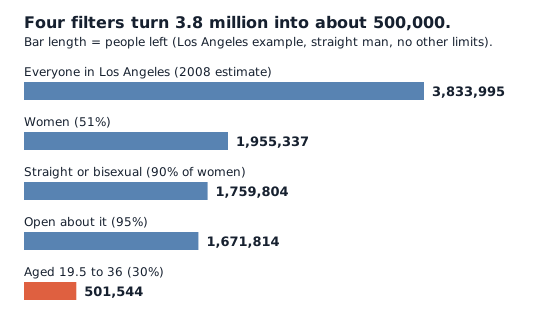
The Drake equation for dating multiplies a population by a chain of fractions: the share you would date, the share who would date you, the age range and any other filters4. A Los Angeles example starts at 3,833,995 people and ends at 501,5444. The 37% rule then says how many candidates to look at before choosing one7.
- The formula
- n = P × ft × fo × fc × A × R: population times a chain of filters4
- Los Angeles example
- 3,833,995 people, four filters, 501,544 left4
- Backus, London
- 10,510 people met his criteria; with attraction, being single and getting along, 265
- The 37% rule
- Look at the first 37% of candidates, choose none, then take the first better than all seen7
- Drake's original
- Frank Drake's 1961 equation for alien civilizations; he suggests N = 10,0001
An astronomer wrote down a handful of factors in 1961, multiplied them together and got a number for how many alien civilizations might be listening1. Decades later a doctoral student at the University of Warwick reused the same shape of equation on a more personal question: how many women in London could he date4? That paper made the calculation famous4. This page runs the dating version with real numbers, shows where it is solid and where it is not, and adds the second piece of math people attach to it, the 37% rule for deciding when to stop looking9.
What is the Drake equation?
The Drake equation is a probabilistic argument for estimating the number of active, communicative extraterrestrial civilizations in the Milky Way3. Frank Drake created it to be part of the agenda for a meeting of experts in West Virginia in 1961, and it serves as a roadmap for astrobiology to this day1. It was formulated as a way to stimulate scientific dialogue at the first scientific meeting on the search for extraterrestrial intelligence, not to produce a headcount3.
Its form is a product of seven factors that, multiplied, give the number of societies broadcasting signals one might pick up1. Drake compares the logic to estimating a university’s undergraduates: multiply the number of freshmen entering each year by the average years spent at school, 4, and you have a good estimate of the student body1. The Drake equation works the same way. A rate of new arrivals is multiplied by how long each one stays.
The inputs are not equally well known. For the original, estimates for N have ranged from 1 to several million1. Drake himself suggests N = 10,000, from one new transmitting society a year, each lasting 10,000 years1. The original meeting’s guesses gave a minimum N of 20 and a maximum of 50,000,0003.
That spread is the first lesson for the dating version. The equation cannot be solved or accurately calculated, but it keeps considerable use for discussion1. A NASA-hosted classroom activity stresses the same point: this is not an equation with an answer that we know2. It simply expresses how many civilized worlds there would be given certain assumptions2. Critics focus on the guessed values of several factors, whose combined effect is an uncertainty so large that firm conclusions cannot be drawn3.
What quantity does the Drake equation calculate?
The original equation estimates N, the number of communicative civilizations in the Milky Way1. The dating adaptation keeps the logic and changes the question. It estimates the number of potential partners in your area who meet a list of conditions4.
How does the Drake equation for dating work?
Peter Backus, a Ph.D. candidate at the University of Warwick, wrote a paper titled “Why I Don’t Have a Girlfriend” that brought the idea wide attention4. His approach was specific to him, and a more general version multiplies six terms: n = P × ft × fo × fc × A × R4.
| Symbol | What it is | Source |
|---|---|---|
| P | The population: your university, city or country, depending on how ambitious you are4 | 4 |
| ft | The fraction of that population you would want to mate with, in broad terms4 | 4 |
| fo | The fraction of those who want to mate with you4 | 4 |
| fc | The fraction open enough about their sexuality to engage in the kind of relationship you want4 | 4 |
| A | The fraction of those remaining who fall within your desired age range4 | 4 |
| R | Factors for any remaining filters you wish4 | 4 |
The age filter can follow the “half your age plus seven” rule4. Everything else is personal.
Worked example: a straight man in Los Angeles
Math Goes Pop runs the equation for a straight man in Los Angeles looking for a woman to date there4. The estimated population of Los Angeles in 2008 was 3,833,9954. Of those, 51% are female, 90% of the women are straight or bisexual, and fc is set conservatively at 95%4.
The age filter needs data. For a 25-year-old man, the socially acceptable age range for a partner is between 19.5 and 364. Census counts for 2000 gave 1,115,974 people between 19.5 and 36 in Los Angeles, roughly 30% of the population4. That is the value of A.
Worked example (our arithmetic): the Los Angeles pool, one filter at a time
| Step | Calculation | People left |
|---|---|---|
| Population P | given | 3,833,9954 |
| Women (51%) | 3,833,995 × 0.51 | 1,955,3374 |
| Straight or bisexual (90%) | 1,955,337 × 0.9 | 1,759,8044 |
| Open about it (95%) | 1,759,804 × 0.95 | 1,671,8144 |
| Aged 19.5 to 36 (30%) | 1,671,814 × 0.3 | 501,5444 |
Setting R = 1 gives n = 501,5444. The first four rows are our intermediate rounding to whole people. R = 1 is probably unrealistic, because a person rarely wants to date a married partner, and personal taste shrinks the pool further4. Each extra filter multiplies the 501,544 by a fraction. Add one filter that keeps 20% and the pool drops to 100,309 (our arithmetic)4.
Results: what did Backus find?
Using data for the parameters he could look up and estimates for the rest, Backus found that 10,510 people met his criteria5. That sounds workable until the last three factors are added: whether these people find him attractive, whether they are single and whether they would get along5. After multiplying those, the number of potential girlfriends dropped to 265.
Worked example (our arithmetic): how little survived the last filters
| Quantity | Calculation | Result |
|---|---|---|
| People meeting his criteria | given | 10,5105 |
| Potential partners after attraction, being single and getting along | given | 265 |
| Share that survived | 26 ÷ 10,510 | about 0.25%, or 1 in 4045 |
Two details matter. First, he put the share of available women he would find attractive at about 5%6. Second, three years after publishing, Backus got married to a friend of a friend he met at a dinner party, and one of his 26 viable partners was two degrees of separation away5. A small pool is not an empty pool, and the calculation is silent on how people actually meet.
Is a different answer possible with the same equation?
Yes. A relationship researcher reran the equation with 20 percent of the pool attractive to her and 20 percent of those finding her attractive, starting from a population above 8 million in New York City, and got 111 potential men6. Mathematician Hannah Fry’s statistical work suggests Backus underestimated many values5. With 20% in place of his 5%, the estimate rises from 26 to 8325.
Check that against the arithmetic. Moving one factor from 5% to 20% multiplies the estimate by 20 ÷ 5 = 4, so 26 becomes 104 (our arithmetic)5. The 832 is 32 times 26, so it must come from more than one changed factor, and only one change is described. Treat 832 as unreplicated. The honest conclusion is the point of the whole exercise: the answer swings by tens of times on guesses, which is exactly what the Drake equation does for aliens.
Is love rarer than aliens?
Backus’s pool and Drake’s N answer different questions, so the comparison is a joke with a number attached. It is still worth doing once. If Drake’s 10,000 civilizations exist among more than 200 billion stars in the Milky Way, the odds of pointing a telescope at a random star and finding one are about 0.000005%5.
Worked example (our arithmetic): the chance for aliens, checked
| Step | Calculation | Result |
|---|---|---|
| Civilizations over stars | 10,000 ÷ 200,000,000,000 | 0.000000055 |
| As a percentage | 0.00000005 × 100 | 0.000005%5 |
The percentage matches the one reported5. The people version is far more favorable in one respect: 501,544 people in the Los Angeles example is a large absolute number even after four filters4. Even Backus’s 26 is a number you could meet. What the equation measures is how fast filters shrink a pool. It is not a forecast of anyone’s love life.
What is the 37% rule in dating?
The second piece of math people attach to dating is the secretary problem, whose solution is known as the 37% rule9. It is also called the marriage problem, the fussy suitor problem and the best choice problem9. The problem is widely believed to have first appeared in the February 1960 issue of Scientific American in Martin Gardner’s column, and Merrill Flood was said to have introduced it in 1949 as the fiancee problem7.
The setup is strict. You see n candidates one at a time in random order9. Each is accepted or rejected the moment you meet them, and a rejected candidate does not come back9. The aim is to land the very best one7.
The failure modes are symmetric. You can stop early and miss the best, or stop late and hold out for a better candidate who does not exist7. The best strategy balances them: look at a fixed fraction of the candidates and choose none, however impressive. Then take the first candidate who beats everyone seen so far7.
Small cases: 2 and 3 candidates
With n = 2 candidates, the best is equally likely to be first or second, so accepting the first gives a 50% chance7. With 3 candidates, accepting the first gives only 1/3 = 33%, because the best is among the last two with probability 2/37. A better rule is to reject the first, then hire the second if she is better than the first and otherwise take the third7. That wins in 3 of the 6 possible orders (counted in the table below, our arithmetic), improving the odds from 33% to 50%7.
Worked example (our arithmetic): the six orders of three candidates, ranked from best to worst
| Order seen (ranks) | Second beats first? | Candidate hired | Outcome |
|---|---|---|---|
| 2, 1, 3 | Yes | rank 1 | Win7 |
| 2, 3, 1 | No, take the third | rank 1 | Win7 |
| 3, 1, 2 | Yes | rank 1 | Win7 |
| 1, 2, 3 | No, take the third | rank 3 | Lose7 |
| 1, 3, 2 | No, take the third | rank 2 | Lose7 |
| 3, 2, 1 | Yes | rank 2 | Lose7 |
Large pools: skip 37%
As the pool grows, the line between looking and leaping lands at 37%: look at the first 37% of candidates, choose none, then leap at the first one better than anyone seen so far7. The strategy also succeeds about 37% of the time7. Vanderbei’s formulation gives the exact ratio: interview the first n/e applicants, where e = 2.71828, and reject them categorically, for a success probability of 1/e8.
A failure rate of 63% (100 minus 37, our arithmetic) sounds bad, but picking at random gives only a 1/n chance, so with 100 candidates the odds are 1%7. By comparison, the 37% guarantee holds no matter how large the pool7. The best candidate is selected about 37% of the time whether there are 100 or 100 million applicants9.
Worked example (our arithmetic): the success curve
For a large pool, skipping a share x of candidates gives a success chance of x × ln(1/x), the large-n form of the formula in Suri’s notes7.
| Share skipped, x | Chance of picking the best |
|---|---|
| 0.1 | 0.2307 |
| 0.2 | 0.3227 |
| 0.3 | 0.3617 |
| 0.368 (1/e) | 0.368, the maximum7 |
| 0.5 | 0.3477 |
| 0.7 | 0.2507 |
| 0.9 | 0.0957 |
How many candidates should you look at first?
The Los Angeles result gives n, and the rule asks you to look at n divided by e before choosing4. That is 501,544 ÷ 2.718 = about 184,508 people (our arithmetic)48. Nobody dates 184,508 people. For Backus’s 26, the cutoff is 26 ÷ 2.718 = about 9.6, so roughly the first 10 people (our arithmetic)58. The rule does not fit a city-sized pool, and that is a signal about the model, not about dating.
The model has stated limits. The number of applicants must be known in advance, which is rarely the case9. The major problem with the model is that in many situations the value of n is unknown4. The dating equation is one way to estimate n4. The solution is also meaningful only if candidates do not know the strategy, because early candidates have no chance at all and might not show up9. Real dating lets you go back, learn and change your criteria, so the 37% rule is a thought experiment about stopping, not a rule of conduct.
Why is the dating pool smaller than it looks?
The practical lesson is in the filters, not the total. When values, beliefs or traits are entered as filters, the size of the field falls drastically6. Filtering out people on options you feel ambivalent about may mean missing some wonderful people6. Backus’s own advice follows from the equation: keep looking, and spend time in places where people who meet your criteria spend time5.
Where to go next
Dividing a prize or a pool fairly is a related puzzle in the math of fair division. Other examples of everyday multiplication and rates are on hidden math in a normal day and calculus in everyday life, and the Math in daily life section collects more.
For the sources behind the stopping rule, read the open lecture notes on optimal stopping and the Princeton paper on the secretary problem. For the alien equation, see the NASA-hosted classroom activity.
Common questions
If this left you with a question, start with How to Divide Something Fairly Between Two People: Math or Math in Everyday Life: 7 Examples From One Normal Day.
Sources
- Drake Equation (SETI 101) · SETI Institute · seti.org · checked October 22, 2026
- Anyone Out There? (Night Sky Network activity) · NASA JPL Night Sky Network, Astronomical Society of the Pacific · nightsky.jpl.nasa.gov · checked October 22, 2026
- Drake equation · Wikipedia · en.wikipedia.org · checked October 22, 2026
- Finding Love with a Modified Drake's Equation · Math Goes Pop! · mathgoespop.com · checked October 22, 2026
- Drake Equation for Love Calculator · Omni Calculator · omnicalculator.com · checked October 22, 2026
- Why Today's Dating Pool Is So Much Smaller Than It Looks (M. Cohen) · Psychology Today · psychologytoday.com · checked October 22, 2026
- Optimal Stopping Rules (S. Suri) · University of California, Santa Barbara, Computer Science · sites.cs.ucsb.edu · checked October 22, 2026
- The Postdoc Variant of the Secretary Problem (R. Vanderbei) · Princeton University · vanderbei.princeton.edu · checked October 22, 2026
- Secretary problem · Wikipedia · en.wikipedia.org · checked October 22, 2026
Published . Every source shows the day it was read. Diagrams: original, by the editors. How we check facts · Report an error.