Story · Math in daily life
Calculus in everyday life: one ordinary morning, five places it hides
Follow one ordinary day and watch calculus run under a cooling coffee, a speedometer, a fenced garden, a bacteria count and a filling tub, with the math shown.
Calculus is the math of change, and a normal morning is full of it: a coffee that cools slower as it nears room temperature, a speedometer that reports a rate, a fence with a best shape, and a tub whose total comes from adding up a flow78.
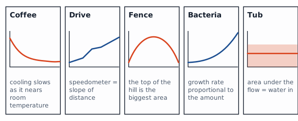
You do not need a whiteboard to meet calculus. You need a kitchen, a car and some patience for what changes. Calculus is the branch of mathematics that studies continuous change7, and almost nothing in a morning stays the same from one minute to the next.
This is one such morning, told in five stops. Each stop names the idea and shows the arithmetic. The derivative rules cheat sheet holds the formulas used here. Short answers first, then the morning. This is the opening page of the daily life section.
What is an example of calculus in real life?
A cup of coffee going cold is the cleanest one: its rate of cooling depends on how far it is above room temperature, so the rate keeps shrinking as it cools1. The same pattern, a rate that depends on the amount present, runs through population growth, interest and radioactive decay3.
What are some real-life applications of calculus?
Think in three families, each one of them a section of this morning. Rates of change cover velocity and acceleration in physics, population growth rates in biology and marginal functions in economics4. Optimization covers the cheapest way to make or package something and the best use of a fixed resource5. Accumulation covers any total built from a changing rate, such as distance from speed or water from a flow67.
The coffee that will not stay hot
You pour a cup at ninety degrees into a kitchen that sits at twenty. For the first minutes it loses heat fast; later it barely seems to change at all. That slowing is the oldest example in the book. Newton’s law of cooling states that the rate of heat loss of a body is directly proportional to the difference in the temperatures between the body and its environment1. A hot cup in a cool room loses heat quickly because the gap is big. As the gap shrinks, so does the rate.
Written as an equation, a rate proportional to a gap is a differential equation (an equation that ties a quantity to its own rate of change), and solving it gives an exponential decrease of the temperature difference over time1. The same family of equations appears wherever a rate depends on the amount present: exponential growth and decay show up in a host of natural applications3, and Newton’s law of cooling is one of them3.
Here is what that looks like with made-up but reasonable numbers. The starting temperature, the room and the cooling constant are all chosen only for illustration.
start 90, room 20, cooling constant 0.05 per minute
T(t) = 20 + 70 · e^(−0.05 t)

t = 0 min    T = 90.0    rate = −3.50 degrees per minute
t = 10 min   T = 62.5    rate = −2.12
t = 20 min   T = 45.8    rate = −1.29
t = 30 min   T = 35.6    rate = −0.78
The rate is the derivative of the temperature. It is always negative because the coffee is cooling, and it shrinks toward zero. That is the first calculus idea of the day: a derivative is a rate of change, and the rate itself can change.
Newton wrote about cooling in 1701, anonymously1. It was the first heat transfer formulation1, and in 2020 two researchers repeated his experiments with modern apparatus and modern data techniques1. The law is not a law of everything, either. It holds well for forced air and pumped liquid cooling1, and it does not describe radiative heat transfer1. It is also more accurate when the working temperature variations are small1. A mug on a kitchen counter sits in still air, so treat the table above as a picture of the shape, not a forecast. A model is a tool with a range, and part of knowing calculus is knowing the range.
Calculus is mostly the habit of asking what is changing, and how fast.
The drive and the speedometer
On the road, calculus sits on the dashboard. Velocity is the rate of change of position, and if you take the derivative of the velocity you get the acceleration, the rate of change of velocity4. Speed is the magnitude of velocity4. A speedometer shows an instantaneous rate, a number for this very instant, while your trip computer shows an average rate over a stretch. The two are different on purpose, and an introductory unit exists just to separate them: the average rate of change is not the instantaneous rate of change4.
average speed = distance / time = 30 miles / (40/60 hour) = 45 mphIf you drove the whole way at exactly the average speed, the speedometer and the trip average would agree. They almost never do, because the speedometer follows the slope of your distance curve at each moment while the average follows only the straight line from start to finish.
Derivatives as rates are not limited to cars. Textbook applications include acceleration and velocity in physics, population growth rates in biology, and marginal functions in economics4. A marginal cost is a derivative of a cost function4.
The idea also solves problems you will not see coming. In a standard related-rates problem, car A starts 500 miles west of the spot where car B starts and drives east, toward that spot, at 35 mph. Car B drives south from the spot, at a right angle, at 50 mph9. How fast is the distance between the cars changing after three hours? The notes work it out9, and you can redo it:
x = distance of A from B's start = 500 − 35·3 = 395
y = distance driven by B          = 50·3      = 150
z² = x² + y² = 395² + 150²        = 178,525,   z = 422.52
2z·z′ = 2x·x′ + 2y·y′   with x′ = −35, y′ = 50
z′ = (395·(−35) + 150·50) / 422.52 = −6,325 / 422.52 = −14.9696
The distance is shrinking at 14.9696 mph, the figure in the notes9. Neither driver sees that number on a dashboard. Calculus makes it computable, because the derivative of a function gives the rate of change of the function9.
The fence you can only build once
At work or at home you often want the best of something with a limit on what you can spend. Optimization is the name for it: one common application of calculus is calculating the minimum or maximum value of a function5. Companies often want to minimize production costs or maximize revenue5, and in manufacturing it is often desirable to minimize the amount of material used to package a product with a certain volume5.
The classic small version is a fence. A rectangular garden uses a wall for one side and fencing for the other three5. In one standard version there are 500 feet of fencing material, and the building takes care of one side10. Two things matter: the quantity you want to maximize, which is the area, and the constraint, which is the fencing you have10. The constraint is the quantity that must be true regardless of the solution10. Solve the constraint for one variable, substitute it into the area, and you get a function of a single variable10.
fence: 2x + y = 500    so   y = 500 − 2x
area:  A(x) = x · (500 − 2x) = 500x − 2x²
A′(x) = 500 − 4x = 0   at   x = 125
then y = 500 − 2·125 = 250,  area = 125 · 250 = 31,250 square feet
The derivative of the area is zero at the top of the hill, where the area stops rising and starts falling. That is where the best shape lives: half as wide as it is long. Nobody guesses that from the numbers alone, and the arithmetic is the whole answer.
A word of honesty about this kind of problem. It is generally one of the more difficult sections for students taking a calculus course10, and the first step is to read the problem very carefully10. It is easy to confuse the thing you optimize with the thing that is held fixed, and a subtle change of wording can change the problem completely10. Slow reading is part of the method, not a sign you are bad at it.
The bacteria nobody counted
At lunch the leftover rice sits on the counter. A population of bacteria is a standard example of exponential growth, because it seems plausible that the rate of population growth would be proportional to the size of the population3. In the language of calculus: the rate of growth is proportional to the current function value3. More bacteria means more reproduction, which means faster growth.
That sentence is a derivative statement: the rate (the derivative) equals a constant times the amount, and the solution of that statement is the exponential function. Money behaves the same way when interest compounds: simple interest is paid once, at the end of the specified time period3, while compound interest is paid multiple times per year, depending on the compounding period3. How loan payments and balances follow from that idea is worked out in the loan payment formula.
Models like these come with a caution. A population really is a whole number of cells, but we are using a continuous function to model what is inherently discrete behavior3. When using exponential growth models, we must always be careful to interpret the function values in the context of the phenomenon we are modeling3.
The tub and the total
In the evening you run a bath. A tub that fills at a steady rate collects water equal to the rate times the time. When the flow changes during the fill, the total is the area under the flow curve. That is what the second half of calculus, integration, is for: integral calculus studies accumulation of quantities and areas under or between curves7.
The connection to the first half is called the net change theorem: when a quantity changes, the new value equals the initial value plus the integral of the rate of change of that quantity6. A rate goes in, a total comes out.
steady fill at 12 liters per minute for 6 minutes:  12 × 6 = 72 liters added
the tub already held 20 liters:                      20 + 72 = 92 liters
Replace the steady twelve with a flow that rises and falls and the multiplication becomes an integral. The idea does not change. A rate is a derivative, a total is an integral, and the net change theorem ties the two together.
What calculus does that earlier math does not
In elementary geometry you describe the slope of a straight line. Calculus can describe the changing slope of a complicated curve7. Geometry gives formulas for the area of triangles and squares, whereas calculus provides a way to find the area of a shape whose boundary is described by a complicated formula7. Calculus has been called the mathematical backbone for solving problems in which variable quantities change with time or another reference value7.
It has an old history. In the late 17th century, Isaac Newton and Gottfried Wilhelm Leibniz each independently formulated infinitesimal calculus, the version built on vanishingly small steps7. The subject exists for what you saw this morning: calculus is the mathematics of how functions change8.
A quick map of what you just saw
| Moment | The question | The idea |
|---|---|---|
| Coffee | How fast is it cooling right now? | Derivative, exponential decay13 |
| Drive | What does the speedometer read? | Derivative of position4 |
| Fence | What shape holds the most? | Optimization510 |
| Bacteria | Why does growth speed up? | Rate proportional to amount3 |
| Tub | How much has it collected? | Integral, net change67 |
Do you have to be a genius?
No. What the textbooks show is a method, not a talent: read the problem carefully, name what changes, name what is fixed, and let the derivative or the integral do the arithmetic10. That is a habit you can practice, and each page in the core ideas section teaches one step of it.
To see a rate turn into money, follow a loan through its monthly payment formula.
If this left you with a question, start with Derivatives in Real Life: Examples With Worked Math or Math in Everyday Life: 7 Examples From One Normal Day.
Sources
- Newton's law of cooling · Wikipedia · en.wikipedia.org · checked October 21, 2026
- 4.3 Separable Equations, Calculus Volume 2 · OpenStax (Rice University) · openstax.org · checked October 21, 2026
- 6.8 Exponential Growth and Decay, Calculus Volume 1 · OpenStax (Rice University) · openstax.org · checked October 21, 2026
- 3.4 Derivatives as Rates of Change, Calculus Volume 1 · OpenStax (Rice University) · openstax.org · checked October 21, 2026
- 4.7 Applied Optimization Problems, Calculus Volume 1 · OpenStax (Rice University) · openstax.org · checked October 21, 2026
- 5.4 Integration Formulas and the Net Change Theorem, Calculus Volume 1 · OpenStax (Rice University) · openstax.org · checked October 21, 2026
- Calculus · Wikipedia · en.wikipedia.org · checked October 21, 2026
- Ch. 1 Introduction, Calculus Volume 1 · OpenStax (Rice University) · openstax.org · checked October 21, 2026
- Calculus I: Rates of Change · Paul's Online Math Notes, Lamar University · tutorial.math.lamar.edu · checked October 21, 2026
- Calculus I: Optimization · Paul's Online Math Notes, Lamar University · tutorial.math.lamar.edu · checked October 21, 2026
Published . Every source shows the day it was read. Diagrams: original, by the editors. How we check facts · Report an error.