How it works · Math in daily life
Derivatives in Real Life: Examples With Worked Math
Where derivatives show up in real life: speed, population, money, best sizes and linked rates. Each example comes with its numbers worked out.
Checked against 6 sources (4 textbook, course or government) · By Ambient Math editors
The short answer. A derivative is a rate of change, so it appears wherever a quantity changes: velocity is the derivative of position, a population's growth rate is the derivative of its size, and marginal cost and revenue are derivatives of cost and revenue1. Optimization finds the best size where a derivative reaches zero2.
- Motion
- Velocity is the rate of change of position; acceleration is the rate of change of velocity1
- Money
- Marginal revenue is the derivative of revenue; about $3 for the 101st dinner in the textbook case1
- Best size
- A garden with 100 ft of fencing peaks at 25 ft by 50 ft, 1250 ft²2
- Caution
- A derivative-based estimate gets worse as the step grows1
You meet derivatives every time a number comes with “per”: miles per hour, dollars per extra item, degrees per minute. Each one is a rate, and a rate is what a derivative measures. Calculus is the study of how functions change4, and the derivative is its tool for asking how fast something is changing right now. Below are six real-life examples, each with the arithmetic done, drawn from OpenStax and Lamar University course material. The rules for computing them live on the derivative rules cheat sheet, and the idea itself is explained on the page about what a derivative is. More everyday scenes sit in the daily life section.
What a derivative measures: average and instant rate
Differential calculus studies instantaneous rates of change and slopes of curves5. An average rate is a change divided by an elapsed time. An instantaneous rate is what that ratio settles to as the time interval shrinks, and it is the derivative1. The two are different on purpose: the textbook objective is to calculate the average rate of change and explain how it differs from the instantaneous rate1.
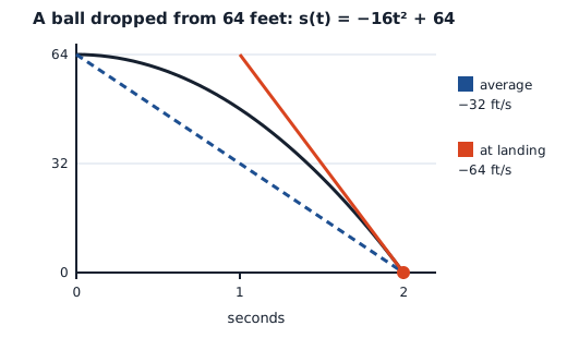
The diagram shows the difference for a falling ball. The dashed line joins the start and the landing and gives the average. The solid line touches the curve at the landing and gives the rate at that instant.
Example 1: speed and acceleration
Velocity is the rate of change of position, and the derivative of velocity is the acceleration, the rate of change of velocity1. Speed is the magnitude of velocity1.
An OpenStax example drops a ball from a height of 64 feet, with height given by s(t) = −16t² + 641. It takes 2 seconds to reach the ground, the instantaneous velocity at landing is −64 ft/s, and the average velocity over the fall is −32 ft/s1.
Worked example (our arithmetic): the dropped ball1
| Step | Calculation | Result |
|---|---|---|
| Time to land | −16t² + 64 = 0, so t² = 4 | t = 2 s1 |
| Velocity function | derivative of −16t² + 64 | v(t) = −32t1 |
| Instantaneous velocity at landing | −32 × 2 | −64 ft/s1 |
| Average velocity over the fall | (0 − 64) / (2 − 0) | −32 ft/s1 |
| Speed at landing | the magnitude of −64 | 64 ft/s1 |
The minus sign only says “downward”. The landing speed is twice the average speed because the ball keeps accelerating on the way down, which is exactly what a straight line from start to finish cannot show.
Example 2: population and growth
The population growth rate is the rate of change of a population, so it is the derivative of the population’s size1. A rate lets you estimate the near future from the present: the new value of a changed quantity equals the original value plus the rate of change times the interval of change1.
The textbook case is a city whose population is tripling every 5 years, currently 10,000, asked for its approximate size 2 years from now1. It answers 18,0001.
Worked example (our arithmetic): the city estimate and a check against growth by tripling1
| Step | Calculation | Result |
|---|---|---|
| Starting size and size in 5 years | 10 and 30 (thousands) | 1 |
| Growth rate at the start | (30 − 10) / (5 − 0) | 4 thousand per year1 |
| Estimate for 2 years ahead | 10 + 2 × 4 | 18 thousand1 |
| If growth keeps tripling every 5 years | 10 × 3^(2/5) | about 15.5 thousand1 |
The textbook warns that the accuracy of this estimate depends on the size of the step1. Over 2 years the straight-line estimate overshoots a steady tripling by about 2.5 thousand (our arithmetic), because the rate used was the starting one and the real growth curve bends. The estimate is fine for small steps and rough for large ones.
Example 3: money, marginal cost and revenue
In business and economics the derivative has its own names. The marginal cost is the derivative of the cost function, and the marginal revenue is the derivative of the revenue function1. The marginal profit is the derivative of the profit function, which is based on the cost function and the revenue function1. In practice the derivative of cost can be read as the change in cost associated with producing one additional item1.
A textbook problem: barbecue dinners sell at a price given by p(x) = 9 − 0.03x for 0 ≤ x ≤ 300, where x is the number sold1. Revenue is then R(x) = x · p(x) = −0.03x² + 9x1. The marginal revenue for the 101st dinner comes out at about $3, while the actual revenue from that dinner is 602.97 − 600 = $2.971. The textbook calls the marginal revenue a fairly good estimate that is easy to compute1.
Worked example (our arithmetic): marginal revenue for the barbecue dinners1
| Dinners sold x | Revenue R(x) = −0.03x² + 9x | Marginal revenue R′(x) = −0.06x + 9 |
|---|---|---|
| 50 | $375.00 | $6.00 per extra dinner1 |
| 100 | $600.00 | $3.00 per extra dinner1 |
| 150 | $675.00 | $0.001 |
| 200 | $600.00 | −$3.001 |
The pattern shows why the derivative earns its keep. Revenue keeps rising while the marginal revenue is positive and peaks where it reaches zero, here at 150 dinners1. Past that, each extra dinner would lower total revenue, because the price falls on every dinner sold.
Example 4: the best size, or optimization
One common application of calculus is calculating the minimum or maximum value of a function2. Businesses use it to push costs down and revenue up, and manufacturers use it to cut the material needed to package a given volume2. Every such problem has a quantity to optimize and an auxiliary condition that must hold2.
The first textbook example is a garden with a rock wall for one side and 100 ft of wire fencing for the other three2. The best garden is 25 ft by 50 ft, with an area of 1250 ft²2. The second example is an open-top box cut from a 24 in. by 36 in. sheet of cardboard by removing a square from each corner2. Its maximum volume is about 1825 in³2.
Worked example (our arithmetic): why the derivative finds the peak2
| Problem | Function | Derivative set to zero | Best result |
|---|---|---|---|
| Garden, 100 ft of fence | A(x) = x(100 − 2x) = 100x − 2x² | A′(x) = 100 − 4x = 0, x = 25 | y = 100 − 2 × 25 = 50, area 25 × 50 = 1,250 ft²2 |
| Garden, test x = 20 | A(20) = 100 × 20 − 2 × 400 | 1,200 ft², lower2 | |
| Garden, test x = 30 | A(30) = 100 × 30 − 2 × 900 | 1,200 ft², lower2 | |
| Box, 24 in. by 36 in. | V(x) = 4x³ − 120x² + 864x | V′(x) = 12x² − 240x + 864 = 0, x = 10 − 2√7 ≈ 4.71 in. | volume ≈ 1,825 in³2 |
The tests either side of x = 25 confirm the peak: moving 5 ft either way loses 50 ft² of area (our arithmetic)2. At the top of a hill the slope is zero, and that is the whole trick.
Example 5: cooling and decay
A cooling drink is a derivative problem in plain sight. Newton’s law of cooling states that the rate of heat loss of a body is directly proportional to the difference in temperature between the body and its environment6. The rate of heat loss is a derivative, so the law is an equation about a derivative. The full treatment, with measured data, is on the page about how fast coffee cools.
Example 6: rates that depend on each other
Sometimes you know how fast one quantity changes and need the rate of another that is tied to it. Lamar University’s notes include a standard case: Car A is west of Car B and starts driving east, toward Car B, at 35 mph, while Car B starts driving south at 50 mph3. After three hours the distance between them is decreasing at a rate of 14.9696 mph3. Nobody reads that number off a dashboard, yet the derivative of the distance gives it. These are called related rates problems, and the notes remind readers that the derivative of a function gives the rate of change of the function3. For the working, see calculus in everyday life.
Why derivatives matter
Algebra and geometry handle fixed shapes and fixed amounts. Calculus can describe the changing slope of a complicated curve, where geometry stops at the slope of a straight line5. It is called the mathematical backbone for solving problems in which variable quantities change with time or another reference value5. In the examples above the derivative did four different jobs: it turned position into speed, population into a growth rate, revenue into a marginal figure and an area function into a best size.
Mistakes with derivative examples
- Mixing average and instant rates. The ball’s average velocity was −32 ft/s and its landing velocity −64 ft/s, so the choice changes the answer by a factor of 21.
- Trusting a linear estimate over a long step. The accuracy of the estimate depends on the step size1, as the city example shows.
- Forgetting the constraint. An optimization problem has a quantity to maximize and a condition that must hold. Dropping the condition gives an unbounded answer2.
- Losing the units. A derivative’s unit is the output unit per input unit: ft/s for the ball, dollars per dinner for revenue1.
- Believing a zero derivative is always a peak. It marks a candidate point, and the textbook method also checks the endpoints of the interval2.
Common questions
Read next
Calculus in everyday life, one morning
Follow one ordinary day and watch calculus run under a cooling coffee, a speedometer, a fenced garden, a bacteria count and a filling tub, with the math shown.
Math in daily lifeMath in Everyday Life: 7 Examples From One Normal Day
Follow one ordinary day through sleep, GPS, groceries, a forecast, a recipe and savings, and see the arithmetic hiding in each, with the numbers sourced.
Math in daily lifeIntegrals in Real Life: Examples With Worked Math
Where integrals show up in real life: fuel burned, distance from speed, a race decided by area, net versus total travel. Each one worked out.
Sources
- 3.4 Derivatives as Rates of Change, Calculus Volume 1 · OpenStax (Rice University) · openstax.org · checked October 21, 2026
- 4.7 Applied Optimization Problems, Calculus Volume 1 · OpenStax (Rice University) · openstax.org · checked October 21, 2026
- Calculus I: Rates of Change · Paul's Online Math Notes, Lamar University · tutorial.math.lamar.edu · checked October 21, 2026
- Ch. 1 Introduction, Calculus Volume 1 · OpenStax (Rice University) · openstax.org · checked October 21, 2026
- Calculus · Wikipedia · en.wikipedia.org · checked October 21, 2026
- Newton's law of cooling · Wikipedia · en.wikipedia.org · checked October 21, 2026
Published . Every source shows the day it was read. Diagrams: original, by the editors. How we check facts · Report an error.