Story · Core ideas
Fundamental Theorem of Calculus Explained: Parts 1 and 2
The Fundamental Theorem of Calculus links derivatives and integrals. Part 1, Part 2, worked examples, when to use each, and when it fails.
Differentiation and integration are inverse operations of each other, and the Fundamental Theorem of Calculus is that fact in 2 parts1. Part 1: the derivative of the area function is the original function. Part 2: a definite integral equals the change in any antiderivative between the endpoints2.
- Needs
- A function that is continuous on the interval3
- Why it matters
- Evaluates integrals without Riemann sums or area formulas2
For centuries there were two separate problems. One asked how steep a curve is at a point. The other asked how much area lies under it. Ancient Greek mathematicians knew how to compute area via infinitesimals, an operation we would now call integration1. Before the discovery of the theorem on this page, it was not recognized that the two operations were related1.
Then someone noticed they undo each other. Calculus as a unified theory of integration and differentiation started from the conjecture and the proof of the fundamental theorem of calculus1. Its very name indicates how central this theorem is to the entire development of calculus2.
Slope and area are opposite jobs, and that is the whole theorem.
The big idea: two operations that reverse each other
The theorem links differentiating a function, which gives its rate of change at every point, with integrating it, which gives the area under its graph or the cumulative effect of small contributions1. Roughly speaking, the two operations can be thought of as inverses of each other1. Intuitively, integration and differentiation are inverse operations which reverse each other1.
Picture a trip. You can see the velocity on the speedometer but cannot look out to see your location1. To visualize the theorem, imagine wanting to know the distance traveled, the net change in position along the highway1. Adding up speedometer readings gives the change in position, and that is the second half of the theorem. The MIT lecture on the theorem draws the same picture: the left side represents speedometer readings4.
The two parts
There are 2 parts to the theorem. The first part deals with the derivative of an antiderivative, while the second part deals with the relationship between antiderivatives and definite integrals1. The terminology on this topic has not been completely standardized, so a textbook may swap the names1.
| Part 1 | Part 2 (the evaluation theorem) | |
|---|---|---|
| Idea | The rate of change of the integral from a fixed start to a variable end is the function itself1 | The integral over a fixed interval is the change in any antiderivative12 |
| What you do | Differentiate an integral2 | Evaluate an antiderivative at the endpoints and subtract2 |
| Output | A function2 | A number3 |
Part 1: the area function and its slope
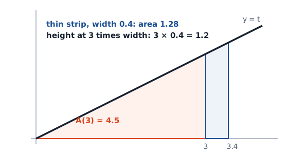
The first fundamental theorem says that the value of any function is the rate of change of its integral from a fixed starting point up to any chosen end point1. That sentence is easier to see than to read. The diagram above plots the line y = t and the area A(x) under it from 0 to x.
At first glance there is something odd about the notation. We have said several times that a definite integral is a number, and here it looks like a function2. The key is that for any particular value of x, the definite integral is a number, so the function returns a number for each x2.
Worked example (our arithmetic): the function f(t) = t and the area function A(x) = the integral of t from 0 to x, which is the area of a triangle2:
| Quantity | Arithmetic |
|---|---|
| A(3), triangle with base 3 and height 3 | ½ × 3 × 3 = 4.52 |
| A(3.4), triangle with base 3.4 and height 3.4 | ½ × 3.4 × 3.4 = 5.782 |
| Strip added: A(3.4) − A(3) | 5.78 − 4.5 = 1.282 |
| Rectangle estimate: width × f(3) | 0.4 × 3 = 1.22 |
| Slope of A near x = 3, strip ÷ width | 1.28 ÷ 0.4 = 3.2, close to f(3) = 31 |
The area strip is close to the width times the height, and the two agree better as the strip narrows1. In the limit, the derivative of the area function exists and equals the original function, so the area function is an antiderivative of the original function1. That is Part 1. It also guarantees that any integrable function has an antiderivative2.
Part 1 with the chain rule
Often the upper limit is not x alone but a function of x. The textbook combines the theorem with the chain rule for this2. Worked example (our arithmetic): the derivative of the integral of cos t from 0 to x²:
| Step | Arithmetic |
|---|---|
| Part 1 on the outside | derivative of the integral of cos t up to u is cos u2 |
| Chain rule: multiply by the derivative of the inside u = x² | 2x2 |
| Result | cos(x²) × 2x = 2x cos(x²)2 |
| Numeric check at x = 1 | 2 × cos(1) = 2 × 0.5403 = 1.0806, and the integral equals sin(x²), whose slope at 1 is the same2 |
Part 2: evaluate an antiderivative
This is the half you use most. Part 2, also known as the evaluation theorem, states that if we can find an antiderivative for the integrand, then we can evaluate the definite integral by evaluating the antiderivative at the endpoints of the interval and subtracting2. Part 2 is perhaps the most important theorem in calculus2. It simplifies the calculation of a definite integral provided an antiderivative can be found by symbolic integration, thus avoiding numerical integration1.
It almost seems too simple that the area of an entire curved region can be calculated by just evaluating an antiderivative at the first and last endpoints of an interval2. Before it, the only tools available were geometric area formulas and limits of Riemann sums, and both approaches are extremely cumbersome2. Remember that the evaluation is always done in the order of upper limit minus lower limit3.
Worked example (our arithmetic): the integral of x² from 1 to 33:
| Step | Arithmetic |
|---|---|
| Antiderivative of x² | F(x) = x³ / 33 |
| Evaluate at the upper limit | F(3) = 27 / 3 = 93 |
| Evaluate at the lower limit | F(1) = 1 / 3 ≈ 0.33333 |
| Subtract, upper minus lower | 9 − 0.3333 = 8.6667, which is 26/33 |
Two practical notes. First, the constant does not matter: the “+ C” term can be left out, because any antiderivative works2. If we had chosen another antiderivative, the constant term would have canceled out, and this always happens when evaluating a definite integral2. Second, the answer can be negative. Area is always positive, but a definite integral can still produce a negative number, a net signed area2. Do not get excited if the lower limit of integration is larger than the upper limit; that happens on occasion and there is nothing wrong with it3.
Most of the work is finding the indefinite integral first3. Once that is done the rest is number crunching3. The same logic is why the power rule and the rest of the derivative rules double as integration facts when read backward.
The engine under Part 1: average value
Part 1 rests on another theorem: a continuous function on a closed interval takes on its average value at some point in that interval2. This is the Mean Value Theorem for Integrals2. It is needed to prove the Fundamental Theorem of Calculus2. The idea is plain: the area under a curve over a width equals the width times some typical height, and that typical height is the average value2.
Worked example (our arithmetic): the function f(x) = 8 − 2x on the interval from 0 to 42:
| Step | Arithmetic |
|---|---|
| Area under the line, a right triangle with base 4 and height 8 | ½ × 4 × 8 = 162 |
| Average value, area divided by width | 16 ÷ 4 = 42 |
| Where the function equals 4 | 8 − 2c = 4, so c = 2, inside the interval2 |
The point c = 2 exists, as the theorem promises2.
Worked example: distance from speed
The second fundamental theorem says that the sum of infinitesimal changes in a quantity adds up to the net change in the quantity1. With velocity as the integrand, the integral is the net change in position14. Worked example (our arithmetic): a speed of v(t) = 6t² meters per second for t from 0 to 3 seconds. The numbers are invented for this example, and the method is Part 22:
| Step | Arithmetic |
|---|---|
| Antiderivative of 6t² | F(t) = 2t³2 |
| At the end, t = 3 | 2 × 27 = 542 |
| At the start, t = 0 | 02 |
| Distance traveled | 54 − 0 = 54 meters24 |
| Sanity check | Top speed 6 × 9 = 54 meters per second; holding 54 for 3 seconds would give 162 meters, so 54 meters is plausible2 |
Quick practice with Part 2
Four more evaluations (our arithmetic), each the antiderivative at the top minus the antiderivative at the bottom3:
| Integral | Antiderivative | Value |
|---|---|---|
| x² from 0 to 3 | x³/3 | 27/3 − 0 = 93 |
| 2x from 1 to 4 | x² | 16 − 1 = 153 |
| cos x from 0 to π/2 | sin x | 1 − 0 = 13 |
| the constant 5 from 0 to 2 | 5x | 10 − 0 = 103 |
Each answer is a number, because definite integrals are numbers while indefinite integrals are functions3. Check the constant case by geometry: a rectangle of height 5 and width 2 has area 10 (our arithmetic)2.
Which part do I use?
| You see | Part | First move |
|---|---|---|
| A variable in the upper limit and a derivative asked for | Part 12 | Replace t with the limit, then multiply by the derivative of the limit2 |
| Numbers on both limits and a value asked for | Part 223 | Find F, then compute F(upper) − F(lower)3 |
| A derivative asked for and a variable in both limits | Part 1, split in 2 | Split the integral at a constant, then apply Part 1 to each piece2 |
| A function with a jump or a hole between the limits | Neither, until you split it | Check continuity first3 |
When the theorem does not apply
The theorem has a condition: the function must be continuous in the interval of integration3. We need to be on the lookout for functions that are not continuous at any point between the limits of integration3. If the point of discontinuity occurs outside of the limits of integration, the integral can still be evaluated3.
Worked example (our arithmetic) of the trap: the integral of 1/x² from −1 to 1. The antiderivative is −1/x, but the function blows up at x = 0, inside the interval3:
| Step | Arithmetic |
|---|---|
| Careless evaluation | F(1) − F(−1) = (−1) − (1) = −23 |
| Reality check | 1/x² is positive everywhere, so an area cannot be −22 |
| Verdict | The theorem does not apply; the integral does not exist in the ordinary sense3 |
A negative answer for a function that is always positive is the red flag. Also note that the corollary version assumes continuity on the whole interval, while the second part of the theorem is slightly stronger1.
Why it mattered, and still does
After tireless efforts by mathematicians for approximately 500 years, new techniques emerged that provided scientists with the necessary tools to explain many phenomena2. Using calculus, astronomers could finally determine distances in space and map planetary orbits2. Everyday financial problems such as calculating marginal costs or predicting total profit could now be handled with simplicity and accuracy2.
Newton and Leibniz explored the relationship during the late 1600s and early 1700s2. The area-function idea is why the integral page can claim an integral undoes a derivative.
Common mistakes
- Putting the limits in the wrong order. It is always the upper limit minus the lower limit3.
- Adding + C and carrying it around. For a definite integral the constant cancels23.
- Using Part 2 across a break. Check continuity between the limits3.
- Forgetting the chain rule in Part 1. When the limit is a function of x, multiply by its derivative2.
- Dropping the absolute value bars on a logarithm. They are required in the evaluation3.
Where to go next
The theorem builds on earlier ideas: the limit, the derivative and the integral. The rest of the core ideas section puts them to work. For the textbook treatment, read OpenStax on the theorem, Lamar University on computing definite integrals and MIT lecture 19.
Common questions
What is the fundamental theorem of calculus in simple terms?
Finding a slope and finding an area are opposite jobs. Build up an area and then differentiate it, and you land back on the curve you started with1. That one fact turns hard area problems into subtraction.
If this left you with a question, start with Derivative rules cheat sheet or What Is a Derivative in Calculus? Simple Explanation.
Sources
- Fundamental theorem of calculus · Wikipedia · en.wikipedia.org · checked October 21, 2026
- 5.3 The Fundamental Theorem of Calculus, Calculus Volume 1 · OpenStax (Rice University) · openstax.org · checked October 21, 2026
- Calculus I: Computing Definite Integrals · Paul's Online Math Notes, Lamar University · tutorial.math.lamar.edu · checked October 21, 2026
- 18.01 Single Variable Calculus, Lecture 19: First Fundamental Theorem of Calculus · MIT OpenCourseWare · ocw.mit.edu · checked October 21, 2026
Published . Every source shows the day it was read. Diagrams: original, by the editors. How we check facts · Report an error.