How it works · Math in daily life
What Is Calculus Used For? Real-Life Uses and Examples
What calculus is used for in real life: speed, growth, profit, medicine and engineering, with worked examples, careers and where the ideas came from.
Checked against 15 sources (13 textbook, course or government) · By Ambient Math editors
The short answer. Calculus measures how fast quantities change and adds up changing amounts. Two problems started it: the slope of a curve at a point and the area under a curve1. It reaches physics, engineering, medicine, economics and any field where a problem can be modeled and an optimal solution is desired14.
- Two core problems
- The tangent (slope at a point) problem and the area under a curve problem1
- Differential calculus
- Velocity and acceleration, the slope of a curve, and optimization14
- Integral calculus
- Area, volume, arc length, center of mass, work and pressure14
- Careers that name it
- Aerospace and electrical engineers, mathematicians and statisticians, actuaries891011
- Worked example
- 500 ft of fence against a building: 250 × 125 encloses the largest area4
On this page
Almost everything that moves, grows, cools or gets used up changes at a rate that is itself changing. A car speeds up, a population gets bigger faster, a hot drink cools quickly and then slowly. Arithmetic handles constant rates. Calculus handles the rest. This guide answers what calculus is used for in plain terms, then shows each use with a worked example: speed, population, profit, distance, the best size for a fence, medicine and decay, the careers that rely on it, and where the ideas came from. The arithmetic is shown so you can check it. For the ideas behind it, the daily life section goes deeper, starting with calculus in everyday life.
What calculus is, in one paragraph
Calculus is the branch of mathematics that studies continuous change14. Differential calculus studies instantaneous rates of change and slopes of curves, and integral calculus studies accumulation of quantities and areas under or between curves14. In the OpenStax calculus text the same idea is one line: calculus is the mathematics of changes in functions7. The two halves are connected: the derivative of the distance is velocity, and the inverse operation takes one from the velocity to the distance13.
What problems does calculus solve?
Two key problems led to the initial formulation of calculus: the tangent problem, or how to determine the slope of a line tangent to a curve at a point, and the area problem, or how to determine the area under a curve1. Both look like geometry. Both are really about change. Rate of change is one of the most critical concepts in calculus1.
The tangent problem: how fast, right now?
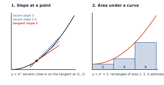
A straight line has one slope. A curve has a different slope at every point, so asking “how fast is it changing right now” needs a new tool. You approximate the rate with a secant line, which is a line through two points of the curve, then slide the second point toward the first. As the second point closes in, the secant lines approach the tangent line1. Instantaneous velocity is the same move applied to a moving object: as t is chosen closer to a, the average velocity becomes closer to the instantaneous velocity1. Average velocity is the change in position divided by the length of the time period1.
The figure shows both problems with the numbers of a textbook example. On the left, secant lines through the point (1, 1) on y = x² have slopes 3 and 2.5 and close in on a tangent with slope 21.
Worked example (our arithmetic): a dropped rock. A rock dropped from a height of 64 ft has height s(t) = −16t² + 64 after t seconds1. Its average velocity just before and just after t = 0.5 s is:
| Interval | Height at start | Height at end | Average velocity |
|---|---|---|---|
| 0.49 s to 0.50 s | 60.1584 | 60.0000 | (60.0000 − 60.1584) / 0.01 = −15.84 ft/s1 |
| 0.50 s to 0.51 s | 60.0000 | 59.8384 | (59.8384 − 60.0000) / 0.01 = −16.16 ft/s1 |
The instantaneous velocity is somewhere between −15.84 and −16.16 ft/sec, and a good guess is −16 ft/sec1. The derivative −32t, evaluated at t = 0.5, confirms −16.
The area problem: how much, in total?
Many quantities in physics, such as quantities of work, may be interpreted as the area under a curve1. Calculus approximates the area by summing the areas of thin rectangles, then lets the rectangles get thinner1. The right side of the figure estimates the area under y = x² + 1 from 0 to 3 with three rectangles of area 1, 2 and 5, an estimate of 81.
The reverse direction works too. Net change adds a rate up into a total: when a quantity changes, the new value equals the initial value plus the integral of the rate of change of that quantity5. It applies to area, distance and volume, to name only a few5.
Worked example (our arithmetic): a drive with a U-turn. A car moves due north at 40 mph between 2 p.m. and 4 p.m., then south at 30 mph between 4 p.m. and 5 p.m.5.
| Leg | Speed × time | Distance |
|---|---|---|
| North, 2 p.m. to 4 p.m. | 40 mph × 2 h | 80 mi north5 |
| South, 4 p.m. to 5 p.m. | 30 mph × 1 h | 30 mi south5 |
| Net displacement | 80 − 30 | 50 mi north5 |
| Total distance | 80 + 30 | 110 mi5 |
At 5 p.m. the car is 50 mi north of its starting position, and between 2 p.m. and 5 p.m. it traveled a total of 110 mi5. To find net displacement you integrate the velocity function over the interval5. A GPS trace and an odometer answer these two different questions, which is why calculus keeps them apart.
How is calculus used in everyday life?
The short version, from a standard calculus text, is that rates of change show up as acceleration and velocity in physics, population growth rates in biology, and marginal functions in economics2. Each of those has a plain-language version.
Speed and acceleration
If you take the derivative of the velocity, you find the acceleration, or the rate of change of velocity2. Newton’s second law of motion is a statement in this language: the derivative of an object’s momentum with respect to time equals the net force upon it14.
Growing populations
A population grows at a rate that depends on its size. In biology, population dynamics starts with reproduction and death rates to model population changes14. For exponential growth, the rate of growth is proportional to the current function value6.
The OpenStax rates section estimates a city’s future population with a derivative: a city of 10,000 people is tripling every 5 years, and the estimate for 2 years from now is 18,0002.
Worked example (our arithmetic): how good is that estimate? The estimate uses the average growth over five years, (30 − 10) / 5 = 4 thousand a year, as the current rate: 10 + 4 × 2 = 18 thousand2. If the city grows exactly exponentially, tripling every 5 years, then 10,000 × 3^(2/5) = 10,000 × 1.5518 = 15,518. A derivative is a linear estimate. It is only as good as the interval is short, and a five-year average is a long interval for a population that is tripling. The textbook itself asks only for an approximate population2.
Cooling, decay and half-life
A cooling drink follows Newton’s law of cooling: the rate of heat loss of a body is directly proportional to the difference in the temperatures between the body and its environment15. Solving that law gives an exponential decrease of temperature-difference over time15. That is why a hot drink loses heat quickly at first and slowly later.
The same shape appears in radioactive decay. From population growth and continuously compounded interest to radioactive decay and Newton’s law of cooling, exponential functions are ubiquitous in nature6. If a quantity decays exponentially, the half-life is the amount of time it takes the quantity to be reduced by half6. Carbon-14 decays at a regular and consistent exponential rate, which is what makes carbon dating possible6. Chemistry uses calculus in a similar way, for example in determining reaction rates14.
Business: marginal cost and profit
The marginal cost is the derivative of the cost function, and the marginal revenue is the derivative of the revenue function2. In economics, calculus allows for the determination of maximal profit by providing a way to easily calculate both marginal cost and marginal revenue14.
Worked example (our arithmetic): the 101st barbecue dinner. In the OpenStax problem, the price is p(x) = 9 − 0.03x dollars when x dinners sell, so revenue is R(x) = x·p(x) = −0.03x² + 9x2. The marginal revenue is R′(x) = −0.06x + 9, so R′(100) = −0.06 × 100 + 9 = 3, and the revenue from the 101st dinner is approximately $32. The exact value is R(101) − R(100) = 602.97 − 600 = $2.972. The marginal revenue is a fairly good estimate in this case and has the advantage of being easy to compute2.
Medicine
In the realm of medicine, calculus can be used in many ways, from predicting the optimal branching angle of a blood vessel to maximize flow, to understanding how quickly a drug is eliminated from a body or how quickly a cancerous tumor grows14. The drug question is exponential decay again, with a half-life in place of a cooling constant.
Getting the most out of a limit: optimization
One common application of calculus is calculating the minimum or maximum value of a function3. Companies often want to minimize production costs or maximize revenue3. In manufacturing, it is often desirable to minimize the amount of material used to package a product with a certain volume3. These problems have a quantity to optimize and a condition that must hold, because we also have some auxiliary condition that needs to be satisfied3.
The classic example is fencing. A field needs a rectangular fence, 500 feet of fencing material is available, and a building on one side means that side needs no fencing4. The dimensions of the field that give the largest area are 250 × 1254.
Worked example (our arithmetic): the fence. Let y be the two short sides and x the long side parallel to the building, so the constraint is x + 2y = 500 and the area is A = x·y4.
| Step | Calculation | Result |
|---|---|---|
| Use the constraint to remove x | x = 500 − 2y | A(y) = (500 − 2y)·y = 500y − 2y²4 |
| Derivative | A′(y) = 500 − 4y | Set to 04 |
| Critical point | y = 500 / 4 | 125 ft4 |
| Long side | x = 500 − 2 × 125 | 250 ft4 |
| Largest area | 250 × 125 | 31,250 sq ft4 |
The check is that the area at either end of the allowed range is zero, so the middle point must be the maximum4.
What real world jobs use calculus?
The U.S. Bureau of Labor Statistics names calculus in its Occupational Outlook Handbook profiles of several fields. Engineers are the clearest case. Aerospace engineers use calculus, trigonometry and other math in their analysis, design and troubleshooting work8. Electrical and electronics engineers must use the principles of calculus and other advanced math to analyze, design and troubleshoot equipment9. Mathematicians and statisticians use statistics, calculus and linear algebra to develop their models and analyses10. Actuaries quantify risk by using the principles of calculus, statistics and probability11.
| Occupation | What the profile ties to calculus | 2025 median pay | Jobs, 2025 | Outlook 2025–35 |
|---|---|---|---|---|
| Aerospace engineers | Analysis, design and troubleshooting8 | $134,960 per year8 | 68,7008 | 8%, much faster than average8 |
| Electrical and electronics engineers | Analyzing, designing and troubleshooting equipment9 | $125,040 per year9 | 297,9009 | 8%, much faster than average9 |
| Mathematicians and statisticians | Models and analyses10 | $105,720 per year10 | 33,50010 | 10%, much faster than average10 |
| Actuaries | Quantifying risk11 | $130,000 per year11 | 31,20011 | 9%, much faster than average11 |
Aerospace engineers design, develop and test aircraft, spacecraft, satellites and missiles8. Actuaries use mathematics, statistics and financial theory to analyze the economic costs of risk and uncertainty11. Industrial engineers, who design systems that move heavy parts within plants, improve hospital wait times or increase vehicle safety, are advised to take algebra, trigonometry and calculus in high school12. Courses for mathematicians and statisticians usually include calculus, differential equations, and linear and abstract algebra10. The same applies to electrical work: students benefit from physics and math, including algebra, trigonometry and calculus9.
Pay, job counts and outlook are the Bureau’s figures for those occupations as a whole, not for the calculus parts of the job. They show where calculus sits in demand, not what the math is worth.
Calculus across the sciences
The reach is wide because the question “how does this change, and what is the total?” is everywhere. Calculus allows one to go from non-constant rates of change to the total change or vice versa, and many times in studying a problem we know one and are trying to find the other14. It is used wherever a problem can be mathematically modeled and an optimal solution is desired14.
- Physics. All concepts in classical mechanics and electromagnetism are related through calculus14. Maxwell’s theory of electromagnetism and Einstein’s theory of general relativity are also expressed in the language of differential calculus14.
- Engineering fields. Vector calculus is used extensively in physics and engineering, especially in the description of electromagnetic fields, gravitational fields and fluid flow14.
- Many disciplines at once. Differential equations relate quantities to their rates of change, and they play a prominent role in engineering, physics, economics and biology14.
- Space and motion. Calculus provides tools, especially the limit and the infinite series, that resolve the paradoxes of motion14.
- Integral applications. Area, volume, arc length, center of mass, work and pressure14.
Beyond one variable, multivariable calculus studies the calculus of functions of two or more variables1.
The history of calculus: where it came from
The main ideas which underpin the calculus developed over a very long period of time indeed, and the first steps were taken by Greek mathematicians13.
| When | Step | Source |
|---|---|---|
| About 450 BC | Zeno of Elea posed problems based on the infinite | 13 |
| About 370 BC | Eudoxus put the method of exhaustion on a scientific basis | 13 |
| Around 225 BC | Archimedes made one of the most significant Greek contributions | 13 |
| 16th century | Mechanics drove mathematicians back to problems such as centres of gravity | 13 |
| October 1666 | Newton wrote a tract on fluxions | 13 |
| By 1675 | Leibniz had settled on his notation | 13 |
| 1690 | Jacob Bernoulli suggested the name integral calculus | 13 |
| 1734 | Berkeley published his Analyst attacking the lack of rigour | 13 |
| 19th century | Cauchy supplied the satisfactory basis | 13 |
Archimedes used the method of exhaustion to approximate the area of a circle, an early example of integration, and his sum for the parabola segment is the first known example of the summation of an infinite series13. Before Newton and Leibniz, Fermat found maxima and minima by calculating when the derivative of the function was 013, and Torricelli and Barrow considered motion with variable speed, where the derivative of the distance is velocity and the inverse operation takes one from the velocity to the distance13.
Newton was the first to apply calculus to general physics, and Leibniz developed much of the notation used in calculus today14. For Newton the calculus was geometrical, while Leibniz took it towards analysis13. Leibniz was very conscious that finding a good notation was of fundamental importance13. The word itself comes from Latin: calculus means “pebble”, a meaning which still persists in medicine14.
Why is calculus so difficult?
Calculus is hard in specific ways, and each one has a remedy.
- It sits on earlier math. The OpenStax text reviews functions first, because it is essential to be familiar and comfortable with these ideas before proceeding to the formal introduction of calculus7. Weak algebra makes every later step shaky.
- Setup comes before calculus. Optimization is generally one of the more difficult sections for students4. The first step in all of these problems should be to very carefully read the problem4, and the constraint is the quantity that must be true regardless of the solution4.
- The logic is subtle. For centuries, mathematicians and philosophers wrestled with paradoxes involving division by zero or sums of infinitely many numbers14. After Berkeley’s attack in 1734, much effort was made to tighten the reasoning, and the really satisfactory basis had to wait for the work of Cauchy in the 19th century13. A topic that took that long to settle is allowed to feel hard.
- Several ideas arrive together. The tangent problem, the area problem and the limit that links them are met in the same course1.
The fix is the same each time: write the quantity, the rate and the constraint in words before touching a formula, and practice the worked examples above with a pencil.
Where to go next
If you want the idea behind the slope, read what is a derivative, then what is a limit and what is an integral. The rules for finding derivatives are on the derivative rules cheat sheet. Calculus also sits under money: the balance on a loan follows the same rate-of-change logic as the cooling drink above, which is the subject of the loan payment formula and how long to pay off a loan. For the primary sources used here, see the OpenStax Calculus Volume 1 preview chapter, the Bureau of Labor Statistics profile of aerospace engineers and the MacTutor history of the calculus.
Common questions
What real world jobs use calculus?
The U.S. Bureau of Labor Statistics names calculus in its profiles of aerospace engineers8, electrical and electronics engineers9, mathematicians and statisticians10 and actuaries11. Industrial engineers are advised to take algebra, trigonometry and calculus in high school12.
What problems does calculus solve?
It solves the tangent problem, finding the slope of a line tangent to a curve at a point, and the area problem, finding the area under a curve1. Both rest on limits. Applications follow: velocity and acceleration, optimization, area, volume and work14.
Why is calculus so difficult?
Several ideas arrive together. Students are expected to be comfortable with functions before the first chapter7, and optimization is one of the harder sections because the setup comes before the calculus4. The logic itself took centuries to settle: a satisfactory basis waited for Cauchy in the 19th century13.
Read next
Calculus in everyday life, one morning
Follow one ordinary day and watch calculus run under a cooling coffee, a speedometer, a fenced garden, a bacteria count and a filling tub, with the math shown.
Core ideasWhat Is a Derivative in Calculus? Simple Explanation
A derivative is the instantaneous rate of change of a function: the slope of its tangent line. Plain meaning, worked examples, notation and when it fails.
Core ideasWhat Is an Integral in Calculus? Area, Sums, Examples
An integral adds up a changing quantity: for a positive function it is the area under the curve. Plain meaning, worked examples, the Fundamental Theorem.
Sources
- 2.1 A Preview of Calculus, Calculus Volume 1 · OpenStax (Rice University) · openstax.org · checked October 21, 2026
- 3.4 Derivatives as Rates of Change, Calculus Volume 1 · OpenStax (Rice University) · openstax.org · checked October 21, 2026
- 4.7 Applied Optimization Problems, Calculus Volume 1 · OpenStax (Rice University) · openstax.org · checked October 21, 2026
- Calculus I: Optimization · Paul's Online Math Notes, Lamar University · tutorial.math.lamar.edu · checked October 21, 2026
- 5.4 Integration Formulas and the Net Change Theorem, Calculus Volume 1 · OpenStax (Rice University) · openstax.org · checked October 21, 2026
- 6.8 Exponential Growth and Decay, Calculus Volume 1 · OpenStax (Rice University) · openstax.org · checked October 21, 2026
- Ch. 1 Introduction, Calculus Volume 1 · OpenStax (Rice University) · openstax.org · checked October 21, 2026
- Aerospace Engineers, Occupational Outlook Handbook · U.S. Bureau of Labor Statistics · bls.gov · checked October 21, 2026
- Electrical and Electronics Engineers, Occupational Outlook Handbook · U.S. Bureau of Labor Statistics · bls.gov · checked October 21, 2026
- Mathematicians and Statisticians, Occupational Outlook Handbook · U.S. Bureau of Labor Statistics · bls.gov · checked October 21, 2026
- Actuaries, Occupational Outlook Handbook · U.S. Bureau of Labor Statistics · bls.gov · checked October 21, 2026
- Industrial Engineers, Occupational Outlook Handbook · U.S. Bureau of Labor Statistics · bls.gov · checked October 21, 2026
- A history of the calculus · MacTutor History of Mathematics, University of St Andrews · mathshistory.st-andrews.ac.uk · checked October 21, 2026
- Calculus · Wikipedia · en.wikipedia.org · checked October 21, 2026
- Newton's law of cooling · Wikipedia · en.wikipedia.org · checked October 21, 2026
Published . Every source shows the day it was read. Diagrams: original, by the editors. How we check facts · Report an error.